Goal Seek Function In Excel For Mac

Excel for Office 365 Excel for Office 365 for Mac Excel 2019 Excel 2016 Excel 2019 for Mac Excel 2013 Excel 2010 Excel 2016 for Mac Excel for Mac 2011 If you know the result that you want from a formula, but are not sure what input value the formula needs to get that result, use the Goal Seek feature. For example, suppose that you need to borrow some money.

Jan 8, 2018 - excel goal seek solve for unknown variables. We show you key Excel formulas and demonstrate how to use them.

Can not insert slide number in powerpoint for mac. You know how much money you want, how long you want to take to pay off the loan, and how much you can afford to pay each month. You can use Goal Seek to determine what interest rate you will need to secure in order to meet your loan goal.

Note: Goal Seek works only with one variable input value. Emulators for raspberry pi. If you want to accept more than one input value; for example, both the loan amount and the monthly payment amount for a loan, you use the Solver add-in. For more information, see.

Step-by-step with an example Let's look at the preceding example, step-by-step. Because you want to calculate the loan interest rate needed to meet your goal, you use the.

The PMT function calculates a monthly payment amount. In this example, the monthly payment amount is the goal that you seek.

Prepare the worksheet • Open a new, blank worksheet. • First, add some labels in the first column to make it easier to read the worksheet. • In cell A1, type Loan Amount. • In cell A2, type Term in Months.

• In cell A3, type Interest Rate. • In cell A4, type Payment.

• Next, add the values that you know. • In cell B1, type 100000. This is the amount that you want to borrow. • In cell B2, type 180. This is the number of months that you want to pay off the loan. Note: Although you know the payment amount that you want, you do not enter it as a value, because the payment amount is a result of the formula. Instead, you add the formula to the worksheet and specify the payment value at a later step, when you use Goal Seek.

• Next, add the formula for which you have a goal. For the example, use the PMT function: • In cell B4, type =PMT(B3/12,B2,B1). This formula calculates the payment amount. In this example, you want to pay $900 each month.

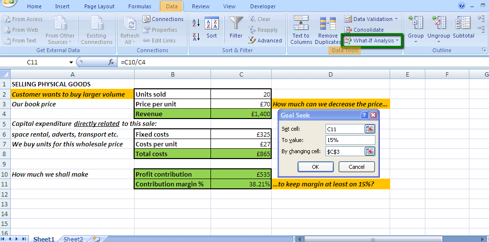
You don't enter that amount here, because you want to use Goal Seek to determine the interest rate, and Goal Seek requires that you start with a formula. The formula refers to cells B1 and B2, which contain values that you specified in preceding steps. The formula also refers to cell B3, which is where you will specify that Goal Seek put the interest rate. The formula divides the value in B3 by 12 because you specified a monthly payment, and the PMT function assumes an annual interest rate. Because there is no value in cell B3, Excel assumes a 0% interest rate and, using the values in the example, returns a payment of $555.56. You can ignore that value for now. Use Goal Seek to determine the interest rate • On the Data tab, in the Data Tools group, click What-If Analysis, and then click Goal Seek.

• In the Set cell box, enter the reference for the cell that contains the formula that you want to resolve. In the example, this reference is cell B4. • In the To value box, type the formula result that you want. In the example, this is -900. Note that this number is negative because it represents a payment.

• In the By changing cell box, enter the reference for the cell that contains the value that you want to adjust. In the example, this reference is cell B3.

Note: Goal Seek works only with one variable input value. If you want to accept more than one input value, for example, both the loan amount and the monthly payment amount for a loan, use the Solver add-in. For more information, see. Step-by-step with an example Let's look at the preceding example, step-by-step.

Because you want to calculate the loan interest rate needed to meet your goal, you use the. The PMT function calculates a monthly payment amount. In this example, the monthly payment amount is the goal that you seek. Prepare the worksheet • Open a new, blank worksheet. • First, add some labels in the first column to make it easier to read the worksheet.

• In cell A1, type Loan Amount. • In cell A2, type Term in Months. • In cell A3, type Interest Rate. • In cell A4, type Payment. • Next, add the values that you know. • In cell B1, type 100000.

This is the amount that you want to borrow. • In cell B2, type 180. This is the number of months that you want to pay off the loan. Note: Although you know the payment amount that you want, you do not enter it as a value, because the payment amount is a result of the formula.