Create A Lookup Table In Excel For Mac

LOOKUP Function (Syntax #1) In Syntax #1, the LOOKUP function searches for value in the lookup_range and returns the value in the result_range that is in the same position. The syntax for the LOOKUP function in Microsoft Excel is: LOOKUP( value, lookup_range, [result_range] ) Parameters or Arguments value The value to search for in the lookup_range. Show account numbers in quickbooks. Lookup_range A single row or single column of data that is sorted in ascending order. The LOOKUP function searches for value in this range.

Result_range Optional. It is a single row or single column of data that is the same size as the lookup_range. The LOOKUP function searches for the value in the lookup_range and returns the value from the same position in the result_range. If this parameter is omitted, it will return the first column of data.

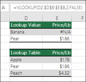
Contents • • • • • • • This Excel Tutorial demonstrates how to use the Excel VLOOKUP Function in Excel to look up a value, with formula examples. VLOOKUP Function Description: The VLOOKUP Function Vlookup stands for vertical lookup. It searches for a value in the leftmost column of a table. Then returns a value a specified number of columns to the right from the found value. It is the same as a hlookup, except it looks up values vertically instead of horizontally. Formula Examples: Example Formula Result Exact Match – Number =VLOOKUP(F5,$B$5:$C$10,G5,H5) 162102 Exact Match – Text =VLOOKUP(F6,$B$5:$C$10,G6,H6) 41681 Closest Match =VLOOKUP(F7,$B$5:$C$10,G7,H7) 133303 Syntax and Arguments: The Syntax for the VLOOKUP Formula is.

= VLOOKUP ( lookup_value, table_array, col_index_num, range_lookup ) Function Arguments ( Inputs ): lookup_value – The value you want to search for. Table_array – The data range that contains both the value you want to search for and the value you want the vlookup to return. The column containing the search values must be the left-most column. Col_index_num – The column number of the data range, from which you want to return a value from.

The most popular of the Excel 2016 lookup functions are HLOOKUP (for. Note that the tip table example in the figure uses an IF function to determine the. Example 4: Create a way of finding the value in the following tables for any row and column heading and value of α. Figure 5 – Table lookup with multiple tables. Here we have three tables like those in Example 1. The first table corresponds to a value of α =.10, the second to α =.05 and the third to α =.01. The approach is the same as.

Range_lookup – TRUE or FALSE. FALSE searches for an exact match. TRUE searches for the nearest match that is less than or equal to the lookup_value. If TRUE is chosen the left-most column (the lookup column) must be sorted ascendingly (lowest to highest). Additional Notes Use the VLOOKUP Function to perform a VERTICAL lookup. The VLOOKUP searches for an exact match ( range_lookup = FALSE) or the closest match that is equal to or less than the lookup_value ( range_lookup = TRUE, numeric values only) in the first row of the table_array. It then returns a corresponding value, n number of rows below the match.